Suppose you want to know the temperature at your house, but you don’t have a thermometer. If one of your neighbours has a weather station, and you live close to your neighbour, you can simply assume that the temperature at your house is the same as your neighbour’s.
What if more than one of your neighbours has a weather station, and all the temperature readings differ? In this case you could take an average of all the measurements. What if you live far away from your neighbours? How would you combine their measurements to obtain an accurate estimate?
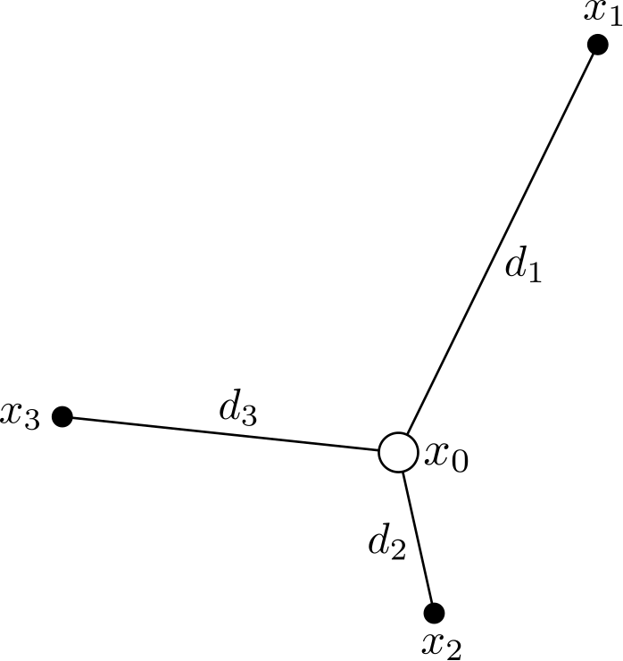
These types of questions can be answered by applying spatial interpolation techniques, which can be explained using the diagram below. The purpose of spatial interpolation is to extend known measurements to areas where no measurements were taken.

The temperature at a central location x0 is needed, but no weather measurements were ever taken there. However, neighbouring locations x1, x2 and x3 all have temperature data available. The simplest way to estimate the temperature at x0 is probably to take the average of the other three; x1, x2 and x3. However, x2 is closer to x0 than x1 is to x0 (i.e. d2 is smaller than d1). Therefore, x2 should have more say than x1 in what the temperature at x0 is.
A slightly more complicated method than mere averaging is inverse distance weighting (IDW), where the amount each neighbour contributes to the central location x0 is determined by the distance between the neighbour and x0. This idea is based on Tobler’s law (the first law of geography): “everything is related to everything else, but near things are more related than distant things“, assuming positive spatial autocorrelation.
Several other spatial interpolation techniques have been developed, including:
- Geostatistical techniques, e.g. Kriging originally developed for mining applications – to determine the structure of gold ore reserves.
- Graphical interpolation, where an area is partitioned based on locations with known measurements, or sample points. The Voronoi polygon is one example where each sample point is located in the middle of a polygon, and all values within each polygon assume the value of the central sample.
- Polynomial techniques including regression and spline interpolation. These techniques involve fitting multivariate mathematical expressions to spatially-distributed data.
- Machine learning, where a neural network is trained on the existing data and then used to estimate or predict data values at unknown locations. An example is given below.
Machine learning spatial interpolation example
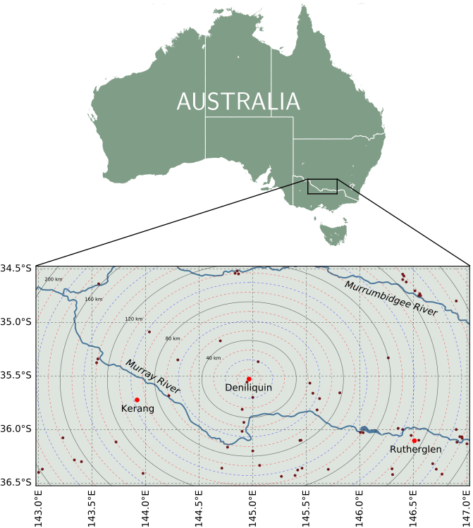
Consider the area around the town of Deniliquin (New South Wales, Australia) shown in the map below. From 1910 to 2018, a total of 71 weather stations (measuring surface air temperature) were active in this area. In this example it will be shown that the temperature record of one station located in Deniliquin can be recreated from the neighbouring stations.

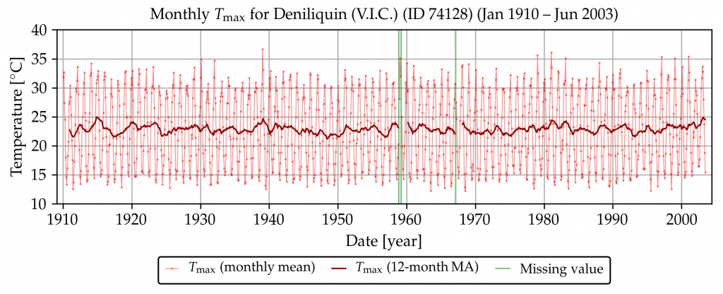
The temperature record used in this example is the monthly mean maximum temperature series shown below.

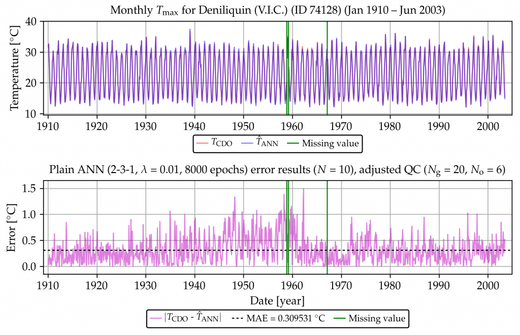
The above record is removed from the record, and an artificial neural network (ANN) is trained on the remaining weather station data. The removed record is then recreated using the trained ANN. The recreated record (in blue) compared with the original one (in red) are shown below, in the top graph. The difference (or error) between the two is also shown below, in the bottom graph.

The same record was also recreated using the IDW method discussed above, and it was found that the ANN method is superior. More technical details of this method are available in this report.

 Jennifer Marohasy BSc PhD is a critical thinker with expertise in the scientific method.
